Optimal Portfolio Choice

Last edited Oct 6, 2026

How diversification, the efficient frontier and the capital allocation line determine what an investor should hold.

This is the theory companion to I Tried to Find the Optimal Investment Portfolio. It follows the progression in my course material: two risky assets, diversification and correlation, the minimum-variance portfolio, many risky assets, a risk-free asset, the capital allocation line, and the tangent portfolio.

The equations are re-typeset from the supplied course material. The figures are original redrawings of the same concepts, computed directly from the worked numbers below rather than reproducing any textbook figure.

1. Two risky assets

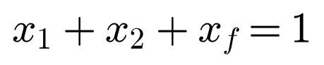
Let x₁ and x₂ be the portfolio shares in Stocks 1 and 2. If the full portfolio is invested:

Expected return

E of R_p equals x1 E of R1 plus x2 E of R2

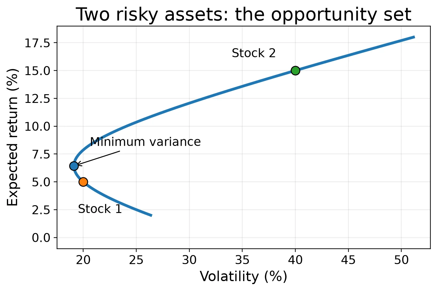
In the course example, Stock 1 has expected return 5% and volatility 20%; Stock 2 has expected return 15% and volatility 40%; and their correlation is 0.2. With x₁ = 0.95 and x₂ = 0.05:

E of R_p equals 0.95 times 5 percent plus 0.05 times 15 percent equals 5.5 percent

Portfolio variance

sigma squared p equals x1 squared sigma1 squared plus x2 squared sigma2 squared plus 2 x1 x2 rho12 sigma1 sigma2

sigma p equals square root of 380.20, approximately 19.5 percent

The portfolio is slightly less volatile than Stock 1 alone even though it contains some of the more volatile Stock 2. That is the diversification effect.

Risk-return curve for two assets showing Stock 1, Stock 2 and the minimum-variance point — The two-risky-asset opportunity set using the course example. The minimum-variance point is the leftmost feasible portfolio.

2. Correlation and diversification

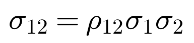
The course expresses the diversification effect as:

Diversification effect equals x1 sigma1 plus x2 sigma2 minus sigma p

0.95 times 20 plus 0.05 times 40 minus 19.5 equals 1.5

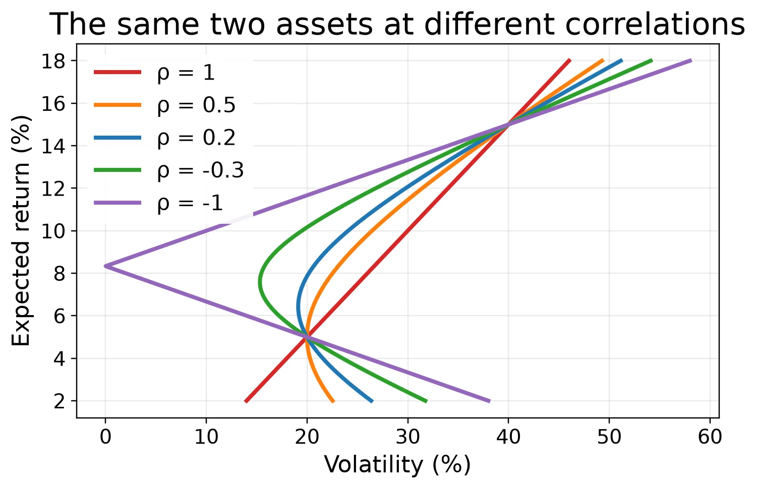
If correlation equals +1, no risk is diversified:

rho12 equals 1 implies sigma p equals x1 sigma1 plus x2 sigma2

As correlation falls, portfolio volatility can fall without changing expected return. At the theoretical limit ρ = −1, suitable weights can create a zero-volatility combination.

The same two assets plotted at five different correlation values, fanning from a straight line at rho=1 to a kinked line at rho=-1 — The same two assets at different correlations. Correlation changes portfolio risk, not the weighted expected return.

3. Negative portfolio shares

The course also allows negative portfolio shares. A negative weight represents a short position. For x₁ = −0.50 and x₂ = 1.50:

x1 equals negative 0.50, x2 equals 1.50, x1 plus x2 equals 1

E of R_p equals negative 0.50 times 5 percent plus 1.50 times 15 percent equals 20 percent

sigma p equals square root of 3460, approximately 58.8 percent

This extends the opportunity set, but in the course example it also produces much higher volatility.

4. The minimum-variance portfolio

Substitute x₂ = 1 − x₁ into portfolio variance and minimize with respect to x₁:

sigma squared p equals x1 squared sigma1 squared plus (1 minus x1) squared sigma2 squared plus 2 x1 (1 minus x1) rho12 sigma1 sigma2

derivative of sigma squared p with respect to x1 equals 0

x1 minimum variance equals, sigma2 squared minus rho12 sigma1 sigma2, over sigma1 squared plus sigma2 squared minus 2 rho12 sigma1 sigma2

x2 minimum variance equals 1 minus x1 minimum variance

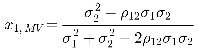
For the course values:

x1 minimum variance approximately 0.857, x2 minimum variance approximately 0.143

E of R minimum variance approximately 6.43 percent, sigma minimum variance approximately 19.1 percent

5. From two assets to many assets

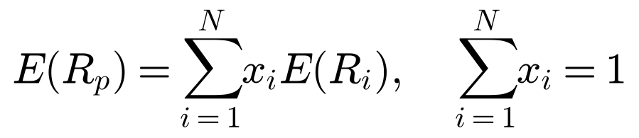
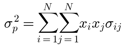
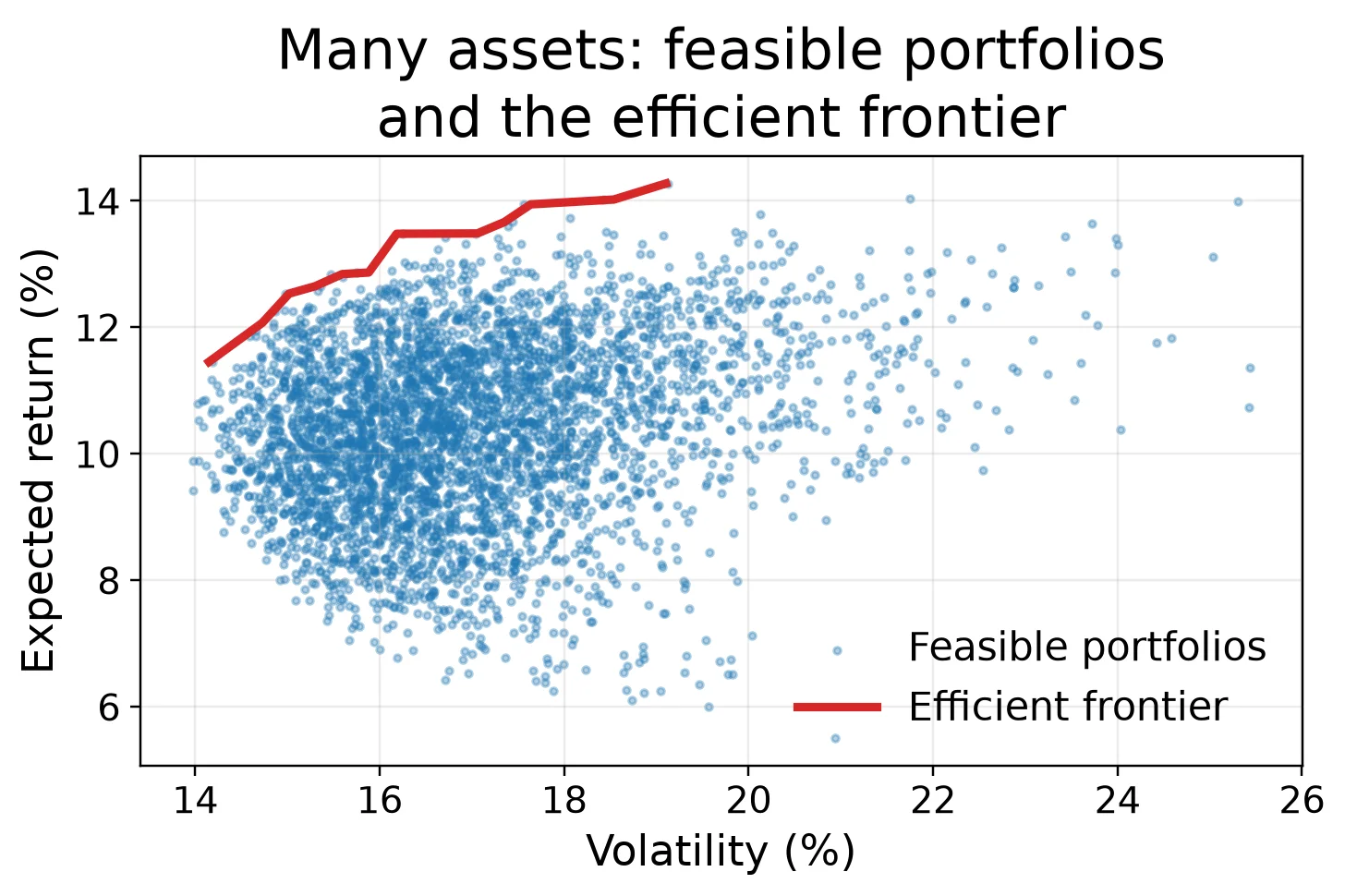
E of R_p equals sum over i of x_i E of R_i, sum of x_i equals 1

sigma squared p equals double sum over i and j of x_i x_j sigma_ij

With many assets, feasible portfolios form a region. Portfolios on the upper boundary above the minimum-variance point are efficient: there is no way to obtain a higher expected return at the same volatility, or lower volatility at the same expected return.

Scatter cloud of simulated feasible portfolios for seven assets with the upper-boundary efficient frontier traced in red — Illustrative feasible portfolios and the efficient frontier. The upper boundary above the minimum-variance point is the part relevant to an efficient investor.

6. Adding a risk-free asset

Let x_B be the share invested in risky portfolio B and 1 − x_B the share in the risk-free asset.

E of R_p equals (1 minus x_B) r_f plus x_B E of R_B

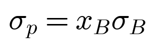
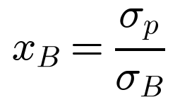
Substituting x_B into expected return gives the capital allocation line:

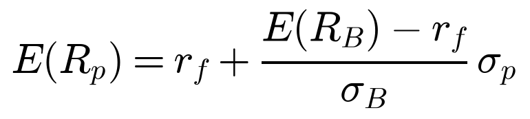
E of R_p equals r_f plus, E of R_B minus r_f over sigma_B, times sigma_p

Increasing x_B increases both expected excess return and volatility proportionally. If x_B exceeds 1, the textbook model represents borrowing at the risk-free rate to obtain leveraged exposure.

7. Sharpe ratio and the tangent portfolio

The slope of the capital allocation line is expected excess return per unit of volatility:

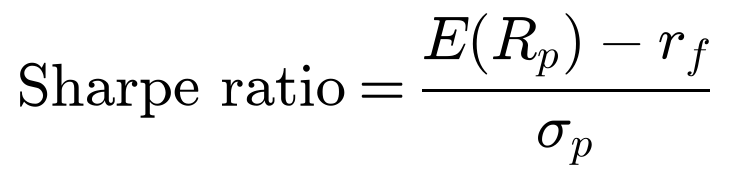
Sharpe ratio equals, E of R_p minus r_f, over sigma_p

For two risky assets plus the risk-free asset, the course writes:

E of R_p equals x1 E of R1 plus x2 E of R2 plus x_f r_f

sigma squared p equals x1 squared sigma1 squared plus x2 squared sigma2 squared plus 2 x1 x2 sigma12

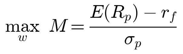
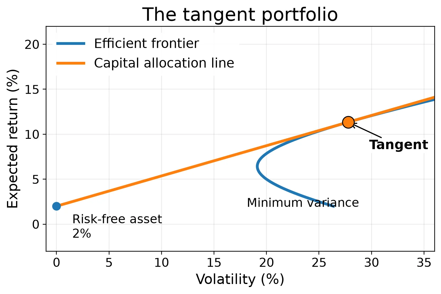
The tangent portfolio is found by maximizing the same reward-to-volatility measure:

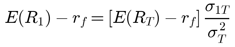
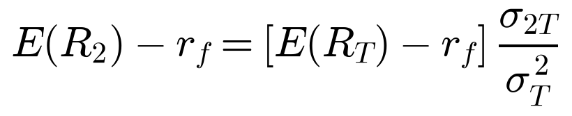
maximize over w, M equals, E of R_p minus r_f, over sigma_p

The course gives these conditions for the solution:

E of R1 minus r_f equals, open bracket E of R_T minus r_f close bracket, times sigma_1T over sigma_T squared

E of R2 minus r_f equals, open bracket E of R_T minus r_f close bracket, times sigma_2T over sigma_T squared

Efficient frontier with a capital allocation line from a risk-free rate of 2 percent, tangent to the frontier at the tangent portfolio — The optimal capital allocation line is the steepest line from the risk-free asset that is tangent to the efficient frontier of risky portfolios. Illustrated here with a 2% risk-free rate on the two-asset example above.

8. The separation result

Once the tangent portfolio T is identified, combinations of the risk-free asset and T lie on the same capital allocation line. If x is the share invested in T:

E of R_C equals (1 minus x) r_f plus x E of R_T

E of R_C equals r_f plus x, open bracket E of R_T minus r_f close bracket

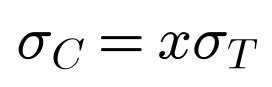
A conservative investor chooses a smaller x; a more risk-tolerant investor chooses a larger x. Under the assumptions of the standard model, both still hold the same tangent portfolio of risky assets.

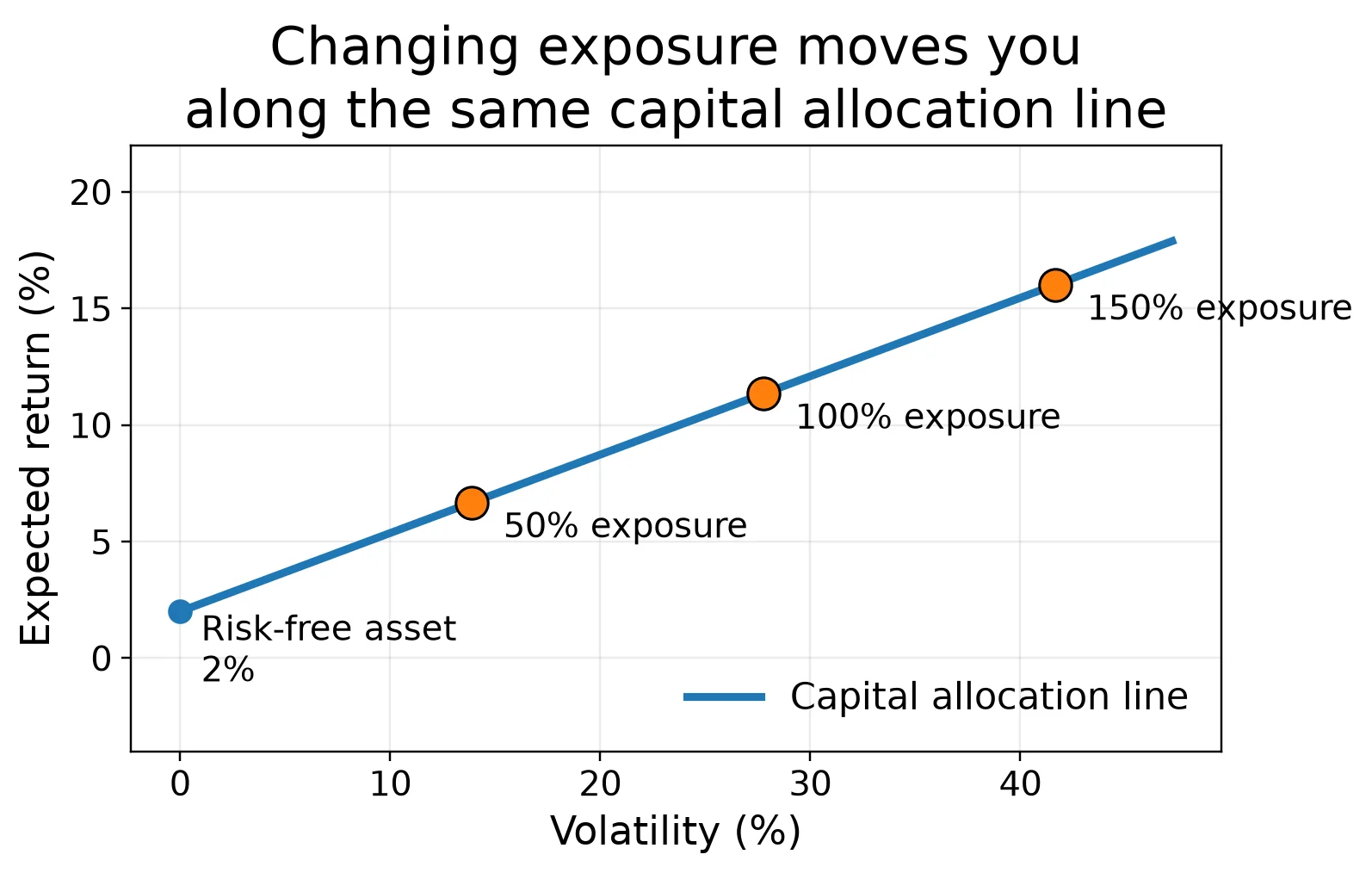
Capital allocation line with three marked points at 50%, 100% and 150% exposure to the tangent portfolio — Changing x moves the investor along the same capital allocation line. Values above 100% correspond to leveraged exposure in the textbook model.

The key result: the tangent portfolio determines the risky-asset mix; investor risk preference determines how much exposure to take to that portfolio versus the risk-free asset.

9. Where the empirical article begins

This theory page deliberately stops where the empirical article begins. The model treats expected returns, volatilities and covariances as inputs. In real data, those quantities have to be estimated.

That is the bridge to I Tried to Find the Optimal Investment Portfolio: the theory tells us what the optimal portfolio would be if the inputs were known; the empirical exercise asks what happens when they have to be estimated.

There is a difference between the optimal portfolio and our estimate of the optimal portfolio.

Sources and attribution

Course: Introduction to Financial Markets and Instruments, Week 40 — Portfolios with two assets. The numerical examples, equations and progression on this page follow the supplied course document.

Textbook reference figures supplied with the course: Berk and DeMarzo, Corporate Finance. They are used here as conceptual references for diversification, the efficient frontier, the capital allocation line, the Sharpe ratio and the tangent portfolio. The figures on this page are independently computed and redrawn, not reproductions of the textbook figures.

Educational material only; not investment advice.